Spectrogram input normalisation for neural networks
In this post, I want to talk about magnitude spectrograms as inputs and outputs of neural networks, and how to normalise them to help the training process.
Introduction: Time-frequency representations, magnitude spectrogram
When using neural networks for audio tasks, it is often advantageous to input not the audio waveform directly into the network, but a two-dimensional representation describing the energy in the signal at a particular time and frequency. A popular time-frequency representation which we will also use here is obtained by the short-time Fourier transform (STFT), where the audio is split into overlapping time frames for which the FFT is computed. From an STFT, we obtain a spectrogram matrix $\mathbf{S}$ with F rows (number of frequency bins) and T columns (number of time frames), where each entry is a complex number. We can take the radius and the polar angle of each complex number to decompose the spectrogram matrix into a magnitude matrix $\mathbf{M}$ and a phase matrix $\mathbf{P}$ so that for each entry we have
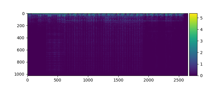
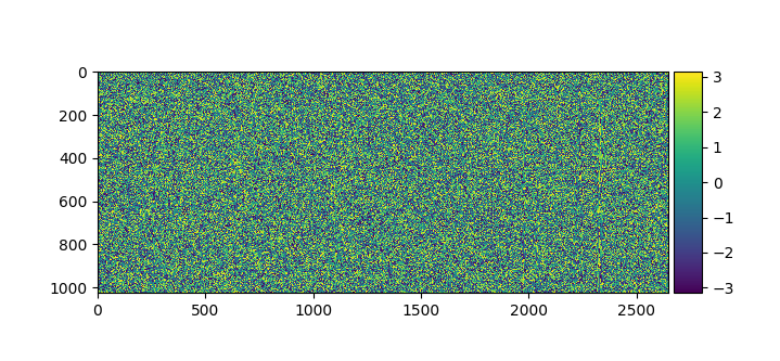
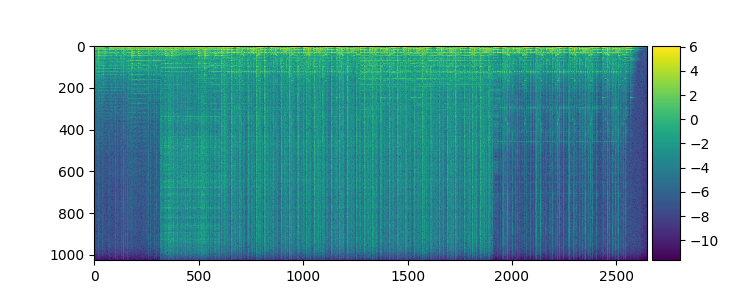
\[S_{i,j} = M_{i,j} * e^{i * P_{i,j}}\]For many audio tasks, only the magnitudes $\mathbf{M}$ are used and the phases $ \mathbf{P}$ are discarded - when using overlapping windows, $ \mathbf{S}$ can be reconstructed from $ \mathbf{M}$ alone, and the phase tends to have a minor impact on sound quality. Here you can see the magnitude and phase for an example song, computed from an STFT with $ N=2048$ samples in each window, and a hop size of 512:
Determining the value range for spectrogram magnitudes
Neural networks tend to converge faster and more stably when the inputs are normally distributed with a mean close to zero and a bounded variance (e.g. 1) so that with the initial weights, the output is already close to the desired one. Similarly, to allow a neural network to output high-dimensional objects, using an output activation function in the last layer that constrains the output range of the network to the real data range can greatly help training and also prevent invalid network predictions. For example, pixels in images are often reduced to a [0,1] interval, and the network output is fed through a sigmoid nonlinearity whose output domain is (0,1).
For these reasons, we need to know the minimum and maximum possible magnitude value in our spectrograms. Since they measure the length of a 2D vector (polar coordinates, their minimum value is zero. For the maximum value of any magnitude, we take a look at how the complex Fourier coefficient for frequency k is computed in an N-point FFT, which ends up in the complex-valued spectrogram:
\[X_k = \sum_{i=0}^{N-1}{x_i \cdot [cos(\frac{2 \pi k n}{N}) - i \cdot sin(\frac{2 \pi k n}{N})]}\]Since the complex part of the product is bounded by 1 in its magnitude, multiplication by the signal amplitude $x_i$ which is between -1 and 1 results in a complex number still bounded by 1 in magnitude. Taking the sum, the maximum for $X_k$ is thus N. When using a window, we multiply a $ w_i$ term to each element in the sum. In the worst case, we have a 1 in magnitude for each entry, so multiplying by each window element gives us the sum of all the window elements as maximum.
Therefore, the range of possible magnitudes resulting from an N-point STFT is: $ [0, \sum_{i=0}^{N-1}{w_i}]$ With a Hanning window, this turns out to be exactly $\frac{N}{2}$. Now we know the value range of magnitudes and could therefore normalise them to a desired range, for example [0, 1]. If we want our model to output audio, we can use a sigmoid function as output activation function, and apply the inverse of this normalisation step, to accelerate learning and ensure that the network outputs are valid.
Gaussianisation to make spectral magnitudes normally distributed
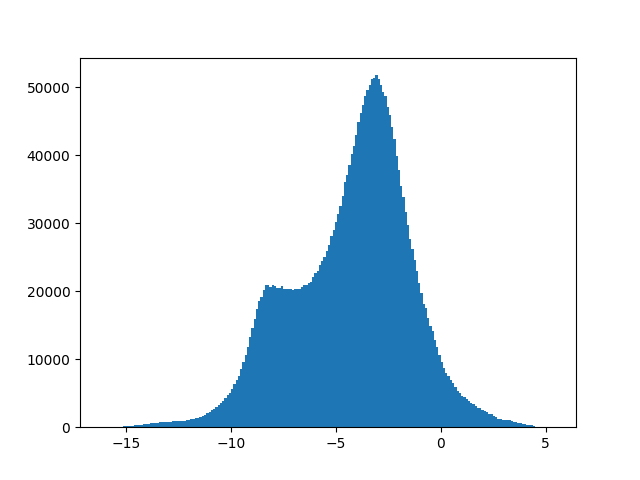
However, the overall distribution of magnitude values is very non-Gaussian, since many entries in the spectrogram are close to zero, creating a very skewed (heavy-tailed) distribution which can impede learning:
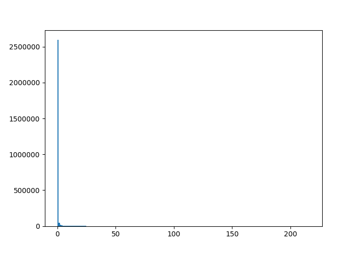
As the plot shows, the magnitudes roughly follow a steep exponential distribution. I will show both an easy, and a more accurate and complex way to make this more normally distributed.
1. Option: A logarithmic transformation
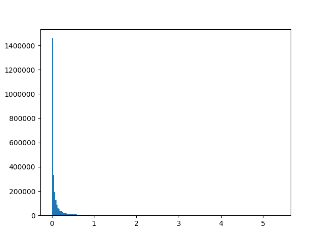
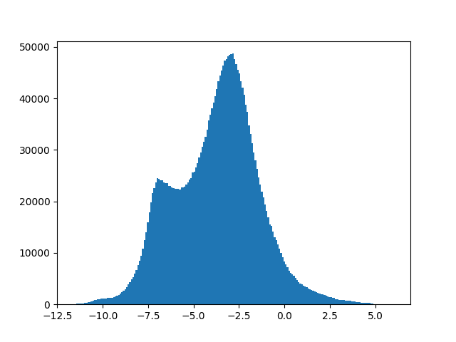
For a roughly exponential distribution, an obvious idea would be to compute $\log(\mathbf{S})$, which is a simple and dataset-independent transformation, to stretch out the near-zero values. However, magnitudes can be zero, and log(0) is undefined! What about if we add a certain positive constant c and compute $\log(\mathbf{S} + c)$? The problem here is that the value of the number critically influences how much low magnitudes close to zero are expanded during transformation - low values of c such as 0.001 lead to great expansion, and vice versa. It is also not immediately clear how to set c to approximate a normal distribution closest. Despite these problems, the transformation at least compresses large values effectively and is used so often that many computing libraries such as Numpy offer the c=1 version with a shorthand called “log1p”, and the inverse “expm1” defined as $\exp{x} - 1$. For our example, we see that c=1 does not change the shape of distribution much at all, while $ c=10^{-7}$ gets us close to a normal distribution:
In general, we see that the closer c is to zero, the more small values are expanded. But how do we set this factor of expansion to make values as close to normally distributed as possible? This is where the Box-Cox transformation comes in!
2. Option: Transformation with Box-Cox
A more advanced method for Gaussianisation is the Box-Cox-Transformation. It comes in two variants: With only one, or with two parameters. We will need the two-parameter version, as it can handle zero values which can occur in our spectrogram. With parameters $ \lambda_1$ and $ \lambda_2$ the Box-Cox transformation is defined as
\[y_i^{(\boldsymbol{\lambda})} = \begin{cases} \dfrac{(y_i + \lambda_2)^{\lambda_1} - 1}{\lambda_1} & \text{if } \lambda_1 \neq 0, \\ \ln{(y_i + \lambda_2)} & \text{if } \lambda_1 = 0. \end{cases}\]Upon closer inspection, we can see similarities to our first option, the logarithmic transformation. $ \lambda_2$ serves the same purpose as the constant c: Making the values non-zero so we can apply further transformations. For $ \lambda_1 = 0$, Box-Cox is even equivalent to our first method and can be seen as an extension of it! The important difference is that the parameters are estimated from data so that the resulting distribution is as close to normally distributed as possible, which is more accurate than a simple log transform with a predefined constant c. I have not come across an implementation that estimates both parameters, though. With the boxcox method from Scipy, we can only estimate $ \lambda_1$, so for our audio example we use $ \lambda_2 = 10^{-7}$ just like in our first method. The best parameter found is $ \lambda_1 = 0.043$, which is very close to zero and therefore a very similar transformation:
Summary
Magnitude spectrograms are tricky to use as input or output of neural networks due to their very skewed, non-normal distribution of values, and because it is hard to find out their maximum value that is needed to scale the value range to a desired interval. The latter is especially important for neural networks that output magnitudes directly, whose training can work better with an output activation function that restricts the network output range to valid values.
The solution is input normalisation: First, transform the values either with a simple $x \rightarrow \log(x+1)$ (first option) or a Box-Cox transformation (second option, more advanced), which should expand low values and compress high ones, making the distribution more Gaussian. Then bring the transformed values into the desired interval. For this we calculate which value 0 and the maximum magnitude are transformed into after applying our particular Gaussianisation, and use this to scale the values to the desired interval.