ICLR 2020 impressions and paper highlights
Having just “visited” my first virtual conference, ICLR 2020, I wanted to talk about my general impression and highlight some papers that stuck out to me from a variety of subfields.
General impressions
I presented our FactorGAN paper at the conference. Like every other paper, we have a quick explainer video, along with an asynchronous chat room to answer questions, and two poster session slots lasting two hours each, where people could spontaneously join into virtual Zoom meetings to discuss the paper.
ICLR organisers did a really good job overall, considering there was so little time to react to the Coronavirus pandemic and to switch from a physical to a virtual conference. Poster sessions were very useful to get to know some people and discuss specific questions about papers. In my experience, they were surprisingly empty oftentimes, but that in turn allowed everyone to participate more easily. It’s really nice that the explainer videos are permanently available to everyone now, which should really help with disseminating all the latest research efficiently.
However, I found it a bit difficult to get to know people in a more relaxed setting. Just like poster sessions, the socials on offer were mostly focused on a specific topic, such as AI for environmental issues. There was a “VR” application called “ICLR Town”, where people can run around with characters in a 2D top-down view and meet up in this virtual space using webcams. While this suited my needs more, there were barely any people online. Maybe such a virtual meeting space should be promoted more and included as a coffee break into the conference schedule- which only featured poster sessions and talks this time.
Finally, I was surprised that poster sessions were not clearly separated according to topic, which made it quite overwhelming to find relevant papers. But overall it was a nice experience and organisers did the best they could considering the circumstances.
Paper highlights
Causality
Connecting deep learning models operating with differentiable operations and loss functions on the one hand with causal learning dealing with discrete graphs on the other hand, is generally a very interesting research direction. I wanted to highlight two papers here.
A Meta-Transfer Objective for Learning to Disentangle Causal Mechanisms
This paper looks at simple two-dimensional distributions $P(A,B)$. The question is: Does A cause B or B cause A? A probabilistic model could estimate the joint by decomposing it into $P(A)P(B|A)$ or $P(B)P(B|A)$. The main idea in this paper: If the model uses the “correct” decomposition that reflects the causal structure, then if the cause changes, adapting the model to this new distribution is fast. Why is that? Let’s assume that A causes B. If we model using the correct decomposition, $P(A)P(B|A)$, and $P(A)$ changes, then $P(B|A)$ stays the same, so only one part of the model needs to be adapted. If we modelled $P(B)P(B|A)$, then BOTH $P(B)$ and $P(B|A)$ would change.
Authors then construct a clever meta-learning objective - a sum of the likelihood of both model variants on the new distribution after training for a certain number of steps. This sum is weighted with the meta-parameter $\gamma$. After meta-training, $\gamma$ indicates which model, and therefore which causal explanation, is most likely the correct one.
This research seems still in its infancy – two-dimensional distributions are clearly not very practically relevant. But the idea of smoothly interpolating between different generative models using meta-learning might prove valuable in the future in more difficult settings!
Neural Causal Induction from Interventions
In this paper, authors employ a deep learning model to estimate the outcomes of particular interventions, and by observing multiple interventions in a row, to predict the structure of the underlying causal graph that generated the observations. This paper also makes use of meta-learning, in that in each meta-iteration, a new causal graph is used, with the aim of obtaining a deep learning model that can predict the causal structure between multiple variables even for new, previously unseen distributions.
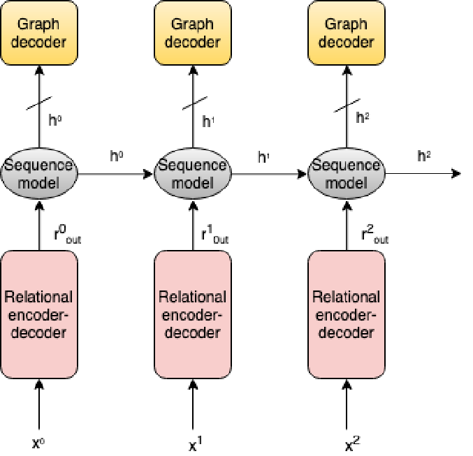
The structure of the neural network is shown above. At each time step, an intervention is performed on one variable, and the encoder takes the resulting $N$ observed variables plus one that indicates which variable was intervened upon. The output is fed to a sequence model that updates its belief state about the causal graph, given all the information (interventions) we have seen so far. Finally, a graph decoder model is trained to output the correct causal graph.
For more detail on these papers and similar papers, check out the workshop on causal learning for decision making.
Classification theory
Your classifier is secretly an energy based model and you should treat it like one
This paper blew me away: Using simple math, it shows very elegantly that a discriminative classifier can also be viewed as an energy-based model, which in turn allows you to detect samples coming from outside the distribution the classifier was originally trained on.
Let’s take a classifier with scalar output $f_{\theta}(x)[y]$ for input $x$ and class index $y$. Class probabilities can be obtained by using the softmax operation, which makes values positive and sum to one over all classes:
$p_{\theta}(y \vert x) = \frac{e^{f_{\theta}(x)[y]}}{\sum_y e^{f_{\theta}(x)[y]}}$.
But the unnormalised outputs can also be used to define an energy based model to define the joint probability over inputs $x$ and labels $y$
$p_{\theta}(x,y) = \frac{e^{f_{\theta}(x)[y]}}{Z(\theta)}$,
where $Z(\theta)$ is the normalising constant that sums up the total energy over the whole $(x,y)$ space. The cool things is - we can now determine the likelihood of an input $p(x)$, by marginalising out $y$ from the above equation, which results in
$p_{\theta}(x) = \frac{\sum_y e^{f_{\theta}(x)[y]}}{Z(\theta)}$.
Notice that the numerator simply contains the sum of exponentiated outputs, which is the denominator in the softmax expression. One can compute $p(y|x)$ to perform classification using the same rules of marginalising out variables, and surprisingly, obtain the exact same formulation of a softmax-based classifier we introduced in the beginning!
Authors then go on and train models as standard classifiers while also maximising the likelihood $p(x)$ at the same time.
The benefits are numerous:
- Obtain good classification accuracy, almost as good as purely discriminative training
- Models can be used to generate new input samples
- Better calibrated classifier output probabilities - NNs are often prone to output probabilities close to 0 or 1, when they should be more uncertain, especially for novel inputs not seen during training. When using the proposed method, samples assigned to a class with a probability of 0.8 would actually end up being from that class 80% of the time.
- Out of distribution detection: Simply check an input example $x$ for its likelihood $p(x)$ - if it is too low, reject the sample and return “I don’t know”
- More robust to adversarial attacks. Even further increased robustness if the input $x$ is first preprocessed by letting the model perturb it into a version $\hat{x}$ that has higher likelihood $p(\hat{x}) > p(x)$ first, thereby “undoing” the adversarial manipulation and restricting classification to input samples that are similar to those seen during training
Towards neural networks that provably know when they don’t know
In a similar vein, this paper calibrates classifier output probabilities by reformulating the conditional $p(y|x)$. This approach assumes samples either come from the “in-distribution” (seen during training), or from a specific “out-distribution”, where the classifier should indicate its complete uncertainty by assigning the same probability to all classes. $p(y|x)$ is then decomposed using Bayes rule:
$p(y \vert x) = \frac{p(y \vert x,i)p(x \vert i)p(i) + p(y \vert x,o)p(x \vert o)p(o)}{p(x \vert i)p(i) + p(x \vert o)p(o)}$
$i$ and $o$ indicate whether a sample comes from the in- or out distribution. $p(y \vert x,i)$ is the classifier of interest, while $p(y \vert x,o)$ is simply set to a uniform distribution over classes, which allows the authors to make uncertainty guarantees. $p(x \vert i)$ and $p(x \vert o)$ are Gaussian mixture models indicating how likely it is to observe this input sample $x$ assuming it’s drawn from the in- or out distribution, respectively.
While the assumption of a specific out-distribution seems limiting, it is very nice to have mathematically proven guarantees for classifier confidences.
Learning with small data, learning representations
Research on how to make deep learning generalise in the face of small datasets has reached a new peak in the last few years. Representation learning, self-supervised learning and meta learning are very popular topics, especially given recent breakthroughs in NLP by models such as BERT, and so ICLR also had a good representation (ha) of papers on these topics.
Current meta-learning approaches are often limited to the few-shot setting, where a model is only updated a few times on a task before it is used to make predictions (e.g. MAML [1], [2]. WarpGrad aims to extend the applicability of meta learning to settings where more adaptation might be needed. Instead of directly learning an update rule for gradient descent, or a model initialisation from which training on a new task should start, it introduces so-called warp layers that essentially transform the optimisation landscape itself. The warp layer parameters can then be meta-learned so that normal SGD methods can more easily converge to good solutions.
For representation learning, Gradients as Features for Deep Representation Learning add another trainable output layer to pre-trained networks that operates on the network’s gradients, in addition to the usual linear output layer that is used to process intermediate activations from the pre-trained network.
In A Mutual Information Maximization Perspective of Language Representation Learning, authors gain very interesting theoretical insight that commonly used representation learning techniques, such as Deep InfoMax or BERT, while not similar at first glance, all end up optimising a version of a common objective that maximises the mutual information between different parts of the input. This paper might turn out to be critical in developing self-supervised learning techniques that work reliably across different input domains (such as text, audio and video).
A critical analysis of self-supervision, or what we can learn from a single image investigates what current computer vision models can learn from very few (even just single) images under current self-supervision techniques, when strong data augmentation is used. The results are quite concerning: Self-supervision techniques currently can not rival standard supervised training even if millions of unlabelled images are used for self-supervision. Also, similar performance with self-supervision can be reached even when using a single image under heavy data augmentation, as this is sufficient to for early network layers to pick up on low-level statistics of natural images. It seems that self-supervision at the moment suffers from the unsolved problem of finding optimisation objectives that actually encourage modelling high-level, semantically meaningful properties of the input.
Audio processing
Due to my background in audio processing, I wanted to specifically highlight two audio related papers.
In Deep Audio Priors, authors propose a new convolution kernel for audio spectrograms. They correctly note that using normal convolutions is well motivated for images, where nearby pixels are strongly correlated. For spectrograms, this also applies to the time dimension, but not to the frequency dimension, where one can find strong dependencies across the whole frequency band. In particular, many sound sources are harmonic, meaning they are comprised of a sine wave with a certain base frequency (fundamental frequency), accompanied by additional sine waves at frequencies which are multiples of the base frequency (caled harmonics). Authors change convolution kernels to reflect this to obtain “harmonic convolution”, which are assigned to attend to a certain base frequency in addition to frequency bins representing the harmonics. Experiments in audio source separation and audio denoising show improved performance over spectrogram-based U-Nets and Wave-U-Net, indicating that such convolutions provide a more suitable “audio prior”.
DDSP - Differentiable Digital Signal Processing This paper integrates many tools from traditional signal processing, such as synthesisers, with deep learning to gain the benefits of both - DSP provides useful building blocks that can realise complicated audio transformations with just a few control parameters, thereby bringing a lot of prior knowledge to bear on the problem at hand, while deep learning can flexibly learn the desired transformation based on the available training data. This can be especially useful for small data scenarios, where DSP tools are not flexible enough and can not make use of the data to improve results, and where standard deep learning models fail since they require much more data since they have to learn everything from scratch.
A final note on transformer efficiency
There was lots of work trying to make transformer models more computationally efficient [1][2][3], since they have a computational complexity of $O(N^2)$ for sequence inputs of length $N$. This is encouraging to see – while their application was mostly limited to processing a few sentences at a time in the domain of NLP, this might allow for modelling long sequences such as audio signals and other time series data.